A user on the RAxML group posted the following including an experimental set-up using a dummy character, observing a high variation in the estimated character weights.
Hello,
I'm interested in using the morphological weight calibration -f u to place fossils [i.e. RAxML's evolutionary placement algorithm] on a molecular tree in comparison to a supermatrix approach [i.e. inferring a tree based on a combined molecular-morphological matrix], but I'm facing two issues.
First, my molecular tree has species that are not represented in the morphological matrix, and RAxML won't weight the morphological alignment when species that have only missing data are present. I have considered adding a dummy character that's coded the same for all species and then dropping the character and its weighting for the final analysis, or calculating the weights on the molecular tree with the species that aren't in the morphological dataset pruned and then using those weights with EPA on the full tree. Before I go basing any sort of downstream analysis on a tree made with morphological weights, I wanted to check if one of these methods is more methodologically sound with the way the morphological weight calibration works.
Second, I ran the weight calibration a few times with the dummy character above to get a sense of what the output would look like, and I've noticed that I seem to get two drastically different sets of weights. I used 1000 replications (-# 1000) and the same random seed for all of them, but I was wondering if producing different weighting schemes was expected. Should I leave the replications where they are and just go with the scheme that has the best likelihood score, or would more replicates converge on a similar weighting scheme?
Thanks for any tips or thoughts you might have on this!
For those who are unfamiliar with EPA, RAxML's in-built evolutionary placement algorithm (Berger & Stamatakis 2010; Berger et al. 2011): EPA finds the optimal place(s) for the fossil, and the weight calibration decreases the decision impact of highly homoplastic characters that do not follow the input tree, typically a molecular-based backbone tree. So, adding naive dummy characters to test what it does, may be not the best idea. To explore, what EPA does (we, e.g., in 2015 used EPA for fossil placement of king fern rhizomes — open access: Bomfleur et al. 2015), and how the estimated weights react from run to run, one could use dummies that
- perfectly fit the (true) tree, Hennig's synapomorphies (i.e., in the original strict sense),
- Dollo-type characters/ homoiologies, and
- such that are randomly distributed.
 |
| Best case, a morphological trait in perfect match with the tree: a synapomorphy (in a strict, Hennigian sense) |
 |
| Note too bad: Dollo-type homoiologies, mutation from black to blue happened twice within the same subtree. |
 |
| Worst-possible case: a morphological trait in total conflict with the tree. |
Being a ML method, EPA considers the input tree's (= mol-inferred tree) branch lengths; characters associated with short branches should have a higher inferred weight variance from run to run. However, if a fossil is only placed based on such uncertain/instable traits, it's placement probabilities will be accordingly split between different alternatives and low for no matter which one (a general tip: make sure that you check the jplace output, not only the RAxML-generated tree regarding ambiguous placements).
Total evidence (supermatrix) trees
When talking about "total evidence" (TE) in the context of fossils, we usually don't include all evidence, we just – well, 'just' means usually a lot of work and research – add a morphological partition to our molecular data set to represent, and, eventually, place, fossil taxa. In the early days of phylogenetic inferences, such TE approaches solved not a few problems (e.g. Wiens 2003–2005, Wiens & Moen 2008 for general background; Wiens et al. 2005, 2006 for applications). These days, they inflict more problems than they might solve, because molecular data have become accessible in increasing large quantity and very good quality resulting in partly trivial, i.e. signal-wise unambiguous phylogenies, while morphological data remained limited, relatively scarce, and complex.
 |
| A Bayesian TE tree of extant and extinct (stars) angiosperms (including some non-angiosperm outgroups), inferred with the purpose of doing a TE dating — which failed, because the ~100 Ma old fossils are resolved by the tree as derived compared to their modern counterparts (from Age of angiosperms, may palaeobotany rest in peace [and pieces], see also Why the emperor has no clothes on pt. 3; the 'supermatrix' used to generate this tree is available on figshare). |
Even if the molecular trees we infer today might still not show exactly the true trees (also because evolution is not necessarily a dichotomous process but involves reticulation and polytomies), we have no way to challenge them or make them "better" by adding morphological data.
On the other hand, having a good molecular tree at hand, facilitates much our handling of the complex, often vague (phylogenetically speaking) morphological data, especially when we want to place fossils.
 |
| Actual signal in a recent angiosperm morphomatrix (Age of angiosperms...) The numbers at the brackets give the bootstrap support for according taxon bipartition, i.e. (alternative) clades in a rooted phylogenetic tree. |
Ignoring molecular data when using morphological traits to place fossils has become a no-go, even if one can still publish pseudo-phylogenies in (allegedly) peer-reviewed, high-impact journals such as Science (Ockham's Razor applied but not used: can we do DNA-scaffolding with seven characters; Surviving parsimonists: just tree-naive or tree-blindfolded). And we need well placed fossils, e.g. for meaningful molecular datings, even somewhat ambiguous ones (Summarizing non-trivial Bayesian tree samples for dating? Just use consensus networks).
Weighting: good, and bad
When done using ML, both EPA, estimating implicit weights, and TE, using the model to counter homoplastic characters, are doing effectively the same for a fossil. A rather trivial fossil, one with relative unambiguous affinities, will be placed the same.
But, the most important result of the molecular revolution was that many aspects of morphologies are poorly sorted, evolutionary speaking. Frankly, we don't need phylogenetic methods to place fossils with obvious affinities. But many fossils provide ambiguous signals, they are not trivial to place (and not only because we miss important traits). Typically, a great number of characters in a morphomatrix support bipartitions that are in conflict with the molecular tree and/or the true tree, while a few match at least aspects of the tree (hence the relative low support for unchallenged molecular clades in morphological data sets). The signal from morpho-partitions is furthermore not very tree-like, morpho-matrices typically have high Delta Values. (Never heard of the Delta Value? Time to read Holland et al. 2002. Curious? Check out the little, platform-independent programme: dist_stats by Markus Göker; early applications: Auch et al. 2006, Göker & Grimm 2008).
- Should we try to infer trees on tree-unlikely matrices?
- More tree-like data forced into trees: a glimpse into the dinosaurs
- A bit of heresy: networks for matrices used in Cladistics studies
- More heretic bits: networks for (more) recent matrices published in Cladistics
- The curious case(s) of tree-like matrices with no synapomorphies
Thus, we also invite bias. If the molecular-inferred topology is not exactly showing the true tree, we may downweigh sites of the morpho-partition (traits) in relative fit with the true tree while upweigh sites in better fit with wrong branches — we propagate error. Total evidence is a double-edge sword, weighting morphological traits for TE inference even more: it may help you better place fossils with ambiguous signal or too much missing data, while giving you inflated supports for subtrees including fossils. The TE tree become even less of a 'total' tree.
This is what happens.
- When you have a split BS of 40 and 39 for fossil X sister to A or B in a morpho-only tree, this tells you that about half of the informative traits say X is related to A and the other half X is related to B.
- In the ML-TE tree, you may already have 60:25 telling you that the traits shared by A and X have a higher tree-fit, e.g. higher proportion of shared derived traits – ideally, a higher phylogeny information content – than those shared by B and X (maybe just shared underived traits).
- If you would use the weighting in a follow-up analysis using a larger data set, this may change to 80:10 split in the TE tree, but this only means that X is likely sister of A under the assumption that only some traits – possibly very few, depending on the weighting scheme – comprise phylogenetic information and all others are irrelevant. Also, the tree used to establish the weights is the true tree.
Branching artefacts: why I never showed a TE tree
The issue of branching artefacts brings us to the main difference between EPA and TE, and why I would always prefer EPA over TE when placing a fossil in a modern-day molecular framework. With EPA, we quickly get probabilities for where in the backbone tree my fossil can be placed; this can be more than one internode!If there are more than one alternative topologies, i.e. partly conflicting, equally probable estimates of the true tree; I can test them all in a quick and consistent fashion.
When going for TE, I only get the single-optimised, possibly biased position. A position that may be influenced by other fossils included in the matrix and inference — biased by taxon sampling. Which can help to prevent (e.g. Wiens 2003) but also invite further branching artefacts (some principal issues: Fossils and networks 1 – Farris and Felsenstein; Large morphomatrices – trivial signal). In case of 'fossil-fossil attraction', weighting may be beneficial again, because it downweighs traits not in fit with the backbone tree. Two fossils that are (due to missing data) identical to each other but showing only evolutionary instable traits, may be resolved as relative well supported sisters in a parsimony or distance TE tree, while support decreases in the ML TE tree, and collapses when using pre-established ML weights. The opposite may also be true. We resolve two fossils as relatively high-supported sisters because they share one or a few higher-weighted traits, which are, however, not so relevant for their part of the tree.
Although I found the papers by Wiens and others very compelling back in the day, I never published TE inferences. When facing the reality of our data, both molecular and morphological, TE (weighted or not) appeared to be pointless.
To place a fossil in a molecular-based framework, just find its optimal position, or equally probable alternative positions.
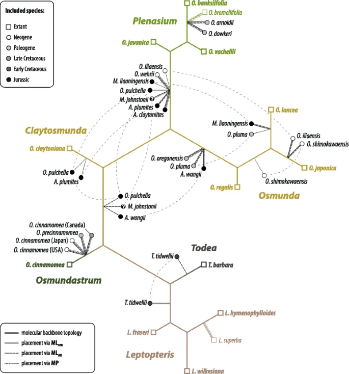 |
| Result of an EPA placing rhizome fossils within the framework of modern-day Osmundaceae (king ferns; Bomfleur et al. 2015, fig. 9) using two flavours of ML weights (only highest probability placements) compared to placement under MP |
And to see how the fossils, the clearly placed and the ambiguous ones, relate to each other (and their current-day relatives, which, naturally, include their descendants), we can only explore the data we have on them: their morphologies.
 |
| A collection of most-parsimonious trees that can be inferred from a pretty unfortunate morphomatrix used to place a fossil, C[astanopsi]s rothwellii, the grey brackets give the synoptical molecular backbone tree (more in Surviving parsimonists...) The graph makes one thing clear: using this trait set to place a fossil is problematic, no matter which method is used. |
And, subsequently, I've been sticking to quick, simple but honest EPA (once it was implemented in RAxML), model-independent distance-based networks (neighbour-nets), and data-display/support consensus networks to further understand the signal/signal quality in the morphological trait sets.
It's always better to fight a somewhat obscure foe – morphological evolution – with shield, bow and dagger than with a double-edged sword – total evidence.
Cited papers (all worth reading, even the older ones)
- Auch AF, Henz SR, Holland BR, Göker M. 2006. Genome BLAST distance phylogenies inferred from whole plastid and whole mitochondrion genome sequences. BMC Bioinformatics 7:350.
- Berger SA, Stamatakis A. 2010. Accuracy of morphology-based phylogenetic fossil placement under Maximum Likelihood. IEEE/ACS International Conference on Computer Systems and Applications (AICCSA). Hammamet: IEEE. p. 1–9.
- Berger SA, Krompass D, Stamatakis A. 2011. Performance, accuracy, and web server for evolutionary placement of short sequence reads under Maximum Likelihood. Systematic Biology 60:291–302. [PDF]
- Bomfleur B, Grimm GW, McLoughlin S. 2015. Osmunda pulchella sp. nov. from the Jurassic of Sweden—reconciling molecular and fossil evidence in the phylogeny of modern royal ferns (Osmundaceae). BMC Evolutionary Biology 15:126.
- Göker M, Grimm GW. 2008. General functions to transform associate data to host data, and their use in phylogenetic inference from sequences with intra-individual variability. BMC Evolutionary Biology 8:86.
- Holland BR, Huber KT, Dress A, Moulton V. 2002. Delta Plots: A tool for analyzing phylogenetic distance data. Molecular Biology and Evolution 19:2051–2059.
- Scotland RW, Steel M. 2015. Circumstances in which parsimony but not compatibility will be provably misleading. Systematic Biology 64:492–504.
- Wiens JJ. 2003. Missing data, incomplete taxa, and phylogenetic accuracy. Systematic Biology 52:528–538.
- Wiens JJ. 2004. The role of morphological data in phylogeny reconstruction. Systematic Biology 53:653–661.
- Wiens JJ. 2005. Can incomplete taxa rescue phylogenetic analyses from long-branch attraction? Systematic Biology 54:731–742.
- Wiens JJ, Fetzner Jr. JW, Parkinson CL, Reeder TW. 2005. Hylid frog phylogeny and sampling strategies for speciose clades. Systematic Biology 54:719–748.
- Wiens JJ, Engstrom TN, Chippindale PT. 2006. Rapid diversification, incomplete isolation, and the "speciation clock" in North American salamanders (genus Plethodon): Testing the hybrid swarm hypothesis of rapid radiation. Evolution 60:2585–2603.
- Wiens JJ, Moen DS. 2008. Missing data and the accuracy of Bayesian phylogenetics. Journal of Systematics and Evolution. Journal of Systematics and Evolution 46:307–314.
No comments:
Post a Comment
Enter your comment ...