In 2015, somebody on ResearchGate posted the following question: “What's the difference between neighbor joining, maximum likelihood, maximum parsimony, and Bayesian inference?” Many answered, a few were ok but a lot repeated common misconceptions. A necessary correction and some further remarks.
I checked the web and found no clear definition on how these various statistical methods differ from each other and how they are estimated. Could anyone elaborate a little bit? (Charles Lorenzo, ResearchGate Q&A, October 2015)
Many said that Neighbour-Joining (NJ) is not a phylogenetic method in contrast to Maximum Parsimony (MP) and Maximum Likelihood (ML) but merely a clustering approach like UPGMA. Which is parsimony-cladistic lore originating in the early years of the Phylogenetic Wars, a series of scientific skirmishes in the 1980s/90s lost by the parsimonists. Another common observation one could make was the expressed tree-naivity by many who responded to the question. Hence, I felt the need to answer, too.
NJ is a cluster algorithm serving as a powerful heuristic to find a distance-based phylogenetic tree
NJ is not “just a clustering algorithm that clusters haplotypes based on genetic distance”, it's a clustering algorithm that is a computational short-cut to quickly infer a phylogenetic tree that either (depending on the settings you use) fulfils the minimum evolution (ME) criterion, which is an optimality criterion closely related to maximum parsimony (see e.g. Felsenstein 2004, p. 159f), or the least-squares (LS) criterion (which is a bit more sophisticated and often better for distance matrices; Felsenstein 2004, p. 148–153).
Just check Wikipedia for “neighbor-joining”, “minimum evolution” and “least-squares” to get the relevant original literature (makes me thinking…should one worry if Wikipedia gets something correct many people dealing in phylogenetics don't?).
 |
| Left: a distance-based phylogenetic tree, a NJ phylogram; right: a UPGMA dendrogram based on the same distance matrix (inferred from Stevenson's 1990 Cycadales matrix). The pink lineage moves one node down in the UPGMA dendogram, Chigua and Microcycas swap places. The left tree, however, shows exactly the phylogenetic relationships, the ‘true tree’, Stevenson coded into his character matrix. |
NJ and UPGMA are both clustering algorithms, but in contrast to NJ, UPGMA will often not come up with a topology that fulfils the ME or LS criterion: the (ultrametric) dendrogram it produces typically doesn't reflect the ‘true tree’, not even in the case of signal-wise trivial matrices. As in the example above, which I will use in this post as illustration. In 1990, Stevenson published a morphological matrix to infer phylogenetic relationships between the genera of the cycads or ”Palmfarne“, ‘palm ferns’, in German (Wp/see Earle's Gymnosperm Database for always up-to-date information; World List of Cycads for all species). In contrast to most other morphological matrices, Stevenson's matrix provided a strongly tree-like, inference-wise trivial signal. He simply encoded the ‘true tree’ (to him) into his matrix. Any method that cannot recover Stevenson's expected phylogenetic relationships such as UPGMA, can hence be considered to be ’non-phylogenetic”. The NJ tree, in contrast, gets it completely right.
[Side-remark: Notably within a blink; Stevenson, relying on parsimony, had to run longer calculations and do quite some post-analysis tweaking to force parsimony into the exact tree he wanted: his Stangeriaceae as sister to Zamiaceae fide Stevenson.]
Weapon's choice
In trivial cases, all phylogenetic inference methods – be they distance-(NJ) or character-based (ML—maximum likelihood, MP—maximum parsimony, BI—Bayesian inference), probabilistic (ML, BI) or not (NJ, MP) or using an explicit substitution model (ML, BI, NJ) or not (MP) – will end up with the same tree. For Stevenson's matrix, the BI-inferred maximum clade credibility (MCC) tree has the same topology as the NJ tree, and the majority rule consensus tree (MRC, quite comb-like) doesn't reject any of the NJ tree's clades. And while there are two equally parsimonious trees, one of them is the NJ tree and the alternative is near-identical, collapsing only the Chigua-Zamia clade (Chigua was back then a freshly erected genus for a unique species of Zamia; but altough trying, Stevenson didn't succeed in scoring their morphological distinctness in his matrix). The ’best-known” ML tree inferred with RAxML is naturally identical to the NJ tree, too.
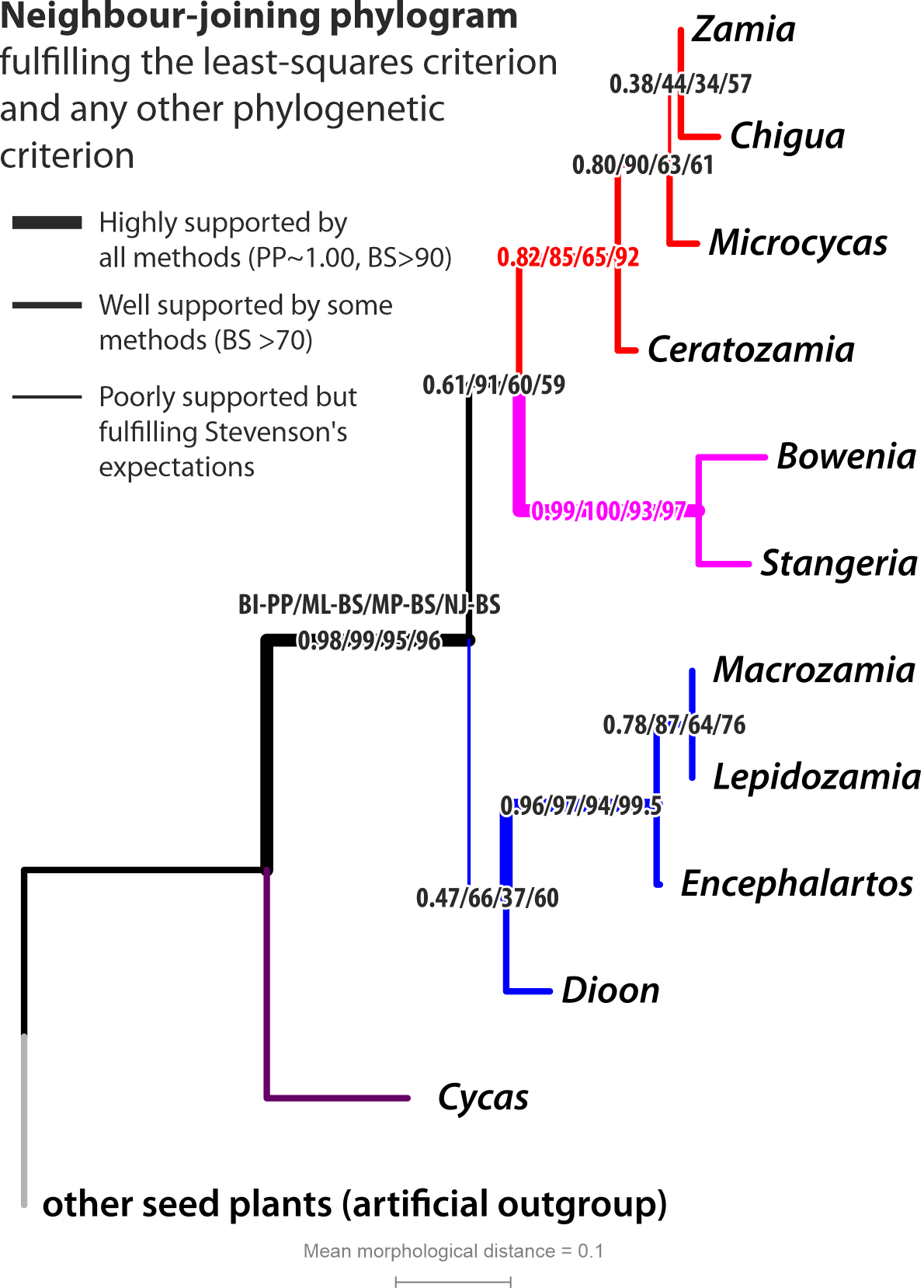 |
| Not so different. NJ tree with branch support from BI (PP—posterior probabilities), ML and MP (BS—non-parametric bootstrapping). Note, ML provided the overall highest branch support for the expected topology, NJ comes second; Bayesian PPs are <<1.00 (quite characteric for morphological data including multistate characters) and MP is the least-discriminative method. |
For Stevenson's matrix, we can say that the NJ tree not only fulfils the distance-based least-squares criterion but also the ML and MP criteria. The NJ cluster algorithm found the most parsimonious and most probable phylogenetic tree solution for the data. A very efficient and extremly quick short-cut. At least for this data matrix.
Just check it for your own data. Science is (should) not (be) about believes (cladistic or other) but about tests. Do you get different NJ and ML trees? Are there splits in the MP trees conflicting with the branches in the NJ, ML or BI trees? Does the ML tree has branches not found in the BI majority rule consensus tree? There may be, because phylogenetic matrices often include non-trivial signals. Some methods are more vulnerable to run into tree-traps put up by these misbehaving signals. And all methods have strengths and weaknesses.
Regarding reliability/ performance, for most (genetic) datasets it's
ML/BI >> NJ > MP
NJ (like a full ME/LS analyses) and MP will always get the wrong tree in the so-called ‘Felsenstein Zone’: When you have long and short branches, the long ones will always attract each other—your inferred tree is biased by the famous ‘long-branch attraction’ (LBA).
Probabilistic inference methods such as ML and Bayesian Inference (BI) have a c. 50% chance to escape LBA.
In other words, if BI/ML disagree with NJ/MP, the latter is likely wrong because of LBA.
But there are more things to keep in mind when different optimality criteria prefer different trees.
The point at which MP and NJ outperform ML/BI
The lower the diversity in your data, the less discriminative ML and BI will be. You won't get necessarily wrong trees, but random ones. ML will still choose one tree, which is however not significantly better than other alternatives and may include numerous branches that receive(d) lower BS support than alternatives not seen in the tree. When using BI, the posterior probabilities (PP) drop below 1.00 and the risk increases for getting trapped in a suboptimum—one can try to avoid that by changing to more parallel runs and deactivate the heating for each chain, e.g. use 10 independent runs with a single chain instead of the standard setting of two × four.
When the rate of change is very low, only parsimony (and NJ provided there's little missing data) will get it.
However, at such a point, you wouldn't settle anymore for the standard phylogenetic tree but use a proper parsimony inference: a median or statistical parsimony network. You inevitably will have to deal with ancestor-descendant pairs, and the standard dichotomous trees can't handle them properly: they assume all ancestors are gone and only their final descendants remained as sisters and cousins. See e.g. this post on the [dormant since 2/11/2020] Genealogical World of Phylogenetic Networks:
For more, search Median network or haplotype network.
PS: In case you have PP <1.00, it's worth to check out the PP consensus network:
 |
| The best (highest Bayesian PP always found for branches seen in the NJ tree) and their next-best topological alternatives. The low PP for the Chigua-Zamia clade reflects lack of discriminate signal in the Stevenson's character matrix (critical data missing for Chigua). |
NJ usually outperforms MP because you have different model choices for estimating the pairwise distance matrix and NJ makes a call rather than coming up with thousands of equally optimal solutions.
[Side-note: It's never a good idea to post-weigh characters to better fit into one tree as done e.g. by TNT, when that very tree has an unknown number of artificial branches to start with. Character-weighting requires a secondary dataset, informing an independently obtained topology, which is then used to down- or upweight individual characters e.g. to better place tips for which we have no secondary data such as fossil taxa in total evidence trees. Still risky, though, why I never opted for total evidence approaches.]
In more cases than not (when you have mid-divergent data) at least the model-based NJ tree, and not rarely even the one based on uncorrected p-distances, will be nearly identical to the ML tree. This NJ/ML-preferred topology will also have the overall highest Bayesian posterior probabilities, but the MP tree may already differ (even when you use the strict consensus tree of all equally parsimonious trees).
But if the NJ starts differing from the ML tree, and becomes more similar to the MP tree, you are approaching the tree space with some Felsenstein zones. Any branch shared by your MP/NJ trees that are in conflict with the ML tree are likely wrong, ‘false positives’, clades that do not reflect monophyletic (in a broad, pre-Hennigian, or narrow, Hennigian, sense: holophyletic) groups.
Most of what I outlined till here you can read in Joe Felsenstein's still-a-good-read book, including the mathematics and many references.
Felsenstein J. 2004. Inferring Phylogenies. Sunderland, MA, U.S.A.: Sinauer Associates Inc.
[Side-note: The only phylogeny textbook, I, having studied geology-palaeontology ending up in plant phylogenetics, ever bought, having been well-advised by a mycologist.]
Missing data and split branch support
NJ is most vulnerable to missing data, ML is the least vulnerable inference. For a simple reason: the more missing data, the less the distance matrix is a reflection of the ‘true tree’. MP easily collapses in the presence of missing data — you don't get too many false positives (“wrong” branches), because you don't get any at all! (Farrisian or Platnickian) Cladists like to point out this as a strength of parsimony but since our objective is to infer a dichotomous tree, not a polytomous comb, using MP tree inference on gappy (swiss-cheese) data matrices is pointless. ML, on the other hand, has been proven to be quite robust against missing data; RAxML, the currently main inference software for ML, has been tested for this extensively. Hence, the widespread use of e.g. the evolutionary placement algorithm implemented in RAxML to place short-reads.
With genetic data, there may still be artefacts when you use swiss-cheese matrices, an example:
BI usually performs as well as ML.
However, you have a higher risk of false positives when you look at the branch support values.
The classic support measure for ML, the non-parametric bootstrapping (BS), can reflect internal signal conflict, expressed as split support patterns in the BS values. For instance, if the preferred branch in the tree has BS support ~ 70 and its alternative, a conflicting branch, a BS support ~ 30 because 70% of all variable sites/ distinct alignment patterns support the branch, and 30% its alternative, then the Bayesian PP will easily converge to 1.00 for the BS =70 alternative. So, when your Bayesian MRC (majority-rule consensus) or MCC (maximum clade credibility) tree conflict with branches in the ML tree, you want to do some ‘exploratory data analysis’ (EDA).
EDA is best-done using networks, e.g. take a look not only at the ML tree but the boostrap consensus network.
Schliep K, Potts AJ, Morrison DA, Grimm GW. 2017. Intertwining phylogenetic trees and networks. Methods in Ecology and Evolution DOI:10.1111/2041-210X.12760 [Open Access]
Examples and more references how and why to do EDA can be found in many of the weekly posts of the (now dormant beauty) Genealogical World of Phylogenetic Networks.
 |
| Maximum likelihood bootstrap (ML-BS) consensus network showing all splits found in 450 pseudoreplicate trees (necessary number determined using extended majority rule bootstop criterion) inferred for Stevenson's Cycadales matrix. Fat edge bundles = branches in the corresponding distance-matrix-based NJ tree. Note that ML (like NJ, MP and BI) fails to unambiguously resolve the sister relationships between close relatives Chigua, Microcycas and Zamia. |
The pointlessness of doing all
For these reasons, you will only find bootstrapped ML trees in most of my post-2005 publications (unless the reviewers-editors insisted). What's the point in inferring a potentially less reliable or oversupporting tree (MP, NJ, BI) in addition to one (ML) that you anyhow will have to prefer when the two (or three) are in conflict with each other?
The main reason people do more than just ML (or BI, if the objective is to get an unambiguously supported tree) is that a lot of elderly (typically male) reviewers are still adhering to the Holy Parsimony Church of Cladistics or feel more confident seeing all done because they themselves are not aware why different optimality criteria and inference algorithms/ heuristics can get different results.
In my work, I dealt with very different data sets, including such with very complex, challenging, non-trivial signals, and never came to the point where the MPTs, the NJ tree or the Bayesian analysis would show anything beyond what could be extracted from the ML tree and the ML-BS consensus network. With one, very notable exception: Towards the tips, when the tree space becomes very flat and probabilistic methods get lost in the indiscriminate tree fog, parsimony can still be informative. In situations where every mutation counts, you go for parsimony-based haplotype network approaches such as statistical parsimony or (my personal favourite) Median networks, full, reduced or filtered. [Reminder: Haplotype networks because standard phylogenetic trees cannot depict ancestor-descendant relationships, and those are what foggies the tree space towards the tips.]
And if you go all the way by doing all: don't just report but try to understand why your ML, MP, BI and NJ (quick-and-easy, so no reason to not add it) prefer different topological alternatives. Embrace, explore the ambiguity, don't ignore it!
Why using distance-based inference in addition to ML (or BI, if you prefer that)
There were however not a few cases, where I used distance matrices (morphology-based, nucleotide-based, ecology-based, handshape-based, reflecting inter-population or inter-individual diversity stemming from intra-genomic variation). Distance methods are not only extremely fast but also versatile, because any sort of data can be translated into a distance matrix and compared without having to infer a tree (or network). And there's is a whole world of different distance measures, just check out the ones implemented by Markus Göker in his little, command-driven and platform-independent programme dist_stats (Auch et al. 2006), which we used in several of our papers showing distance-based graphs and correlations to investigate phylogenetic relationships (e.g. Göker & Grimm 2008—open access).
But, distance matrices are best-analysed (and -visualised) not using the NJ algorithm, but the neighbour-net algorithm
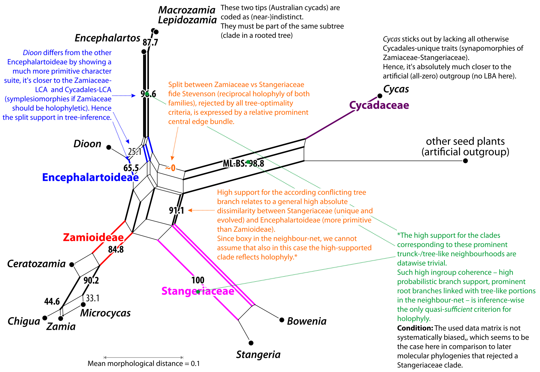 |
| Neighbour-net splits graph based on Stevenson's matrix, numbers give the BS support of the corresponding branch under ML. Only the combination of overall (dis-)similarity patterns using a 2-dimensional graph: a simple, planar, (meta-)phylogenetic network and phylogenetic tree inference(s) allows one to interpret neighbourhoods and clades towards holophyly (or monophyly in a broader sense). |
Originally described (and naturally ignored by biologists) in (peer-reviewed) bioinformatic conference proceedings in 2002, it was made known to the biological public two years later under pretty much the same title.
Bryant D, Moulton V. 2004. Neighbor-Net: An agglomerative method for the construction of phylogenetic networks. Molecular Biology and Evolution 21:255–265. [first introduced in: Bryant D, Moulton V. 2002. NeighborNet: an agglomerative method for the construction of planar phylogenetic networks. In: Guigó R, and Gusfield D, eds. Algorithms in Bioinformatics, Second International Workshop, WABI. Rome, Italy: Springer Verlag, Berlin, Heidelberg, New York, p. 375–391.]
[Technical note: The associated software anyone could have been using was SplitsTree (Huson 1998; Huson & Bryant 2006). A Java-based, platform-independent freeware, with SplitsTree4 being my other good friend in battle (hand-in-hand with RAxML). While the repainted SplitsTree5 turned out to be an “evolutionary dead-end” SplitsTree4's functionality is about to be fused with that of Dendroscope 3 (Huson & Scornavacca 2012). The new crossover still in testing and development, SplitsTree6, is already available for early-access download.]
Unfortunately, a quick and simple method largely ignored to this very day. Although the resultant splits graphs can show you things about your data beyond your ML trees. And more often than not connect finely with what you see in the (ML-)BS consensus networks.
Felsenstein J. 2004. Inferring phylogenies. Sunderland, MA, U.S.A.: Sinauer Associates Inc. ISBN: 9780878931774. [GoogleBooks; Publisher]
Huson DH. 1998. SplitsTree: analyzing and visualizing evolutionary data. Bioinformatics 14:68–73.
Huson DH, Bryant D. 2006. Application of phylogenetic networks in evolutionary studies. Molecular Biology and Evolution 23:254–267. Huson DH, Scornavacca C. 2012. Dendroscope 3: an interactive tool for rooted phylogenetic trees and networks. Systematic Biology 61:1061–1067.
No comments:
Post a Comment
Enter your comment ...